Valuation of Stock Option Using Balck-Scholes Model - Part 5
May 19, 2026
5.1 Valution of Dilutive Corporate Options (Warrants and Employee Stock Options)
The exercise of a regular exchange-traded call option has no operational effect on the underlying number of a company’s shares outstanding. If the writer of a regular option does not own the shares, they must purchase them in the open market and deliver them to the option holder at the strike price.
However, warrants and employee stock options behave differently. Their exercise forces the company to issue entirely new shares of stock and sell them to the option holder for the strike price $K$. Because this strike price is lower than the prevailing market price, the transaction naturally dilutes the equity interest of existing shareholders.
How should potential dilution affect the way we value outstanding options? The answer is that it should not. Assuming markets are efficient, the current market stock price will already reflect the potential dilution from all outstanding warrants and employee stock options.
5.1.1 Evaluating the Cost of a New Options Issue
Consider the situation where a company is contemplating a brand-new issue of warrants or employee stock options. We want to calculate the true cost of this issue, assuming there are no immediate compensating benefits to the firm.
Let's define our initial parameters:
- $N$: The number of existing shares outstanding.
- $S_0$: The current price per share before the issue.
- $M$: The number of new warrants contemplated.
- $K$: The fixed strike price per warrant.
- $T$: The maturity time of the warrants.
The total market value of the company’s equity today is $N S_0$. This aggregate value does not change purely as a result of the warrant announcement. Let's assume that without the warrant issue, the market share price would grow to $S_T$ at maturity. This implies that the total terminal value of the company's equity assets at time $T$ must equal $N S_T$.
If the warrants finish in-the-money and are exercised at time $T$, the company receives a direct cash inflow equal to the total strike price paid, $M K$. This capital infusion increases the total value of the firm's equity to:
5.1.2 Diluted Share Price and Holder Payoff
Because the warrants were exercised, this new pool of total equity value must now be distributed among $N + M$ shares. Therefore, the actual diluted share price immediately following exercise becomes:
Consequently, the net payoff to an individual warrant holder upon exercise is the difference between this diluted post-exercise share price and the strike price $K$ they paid to enter:
We can simplify this fraction algebraically by finding a common denominator for $K$:
The $+M K$ and $-M K$ terms cancel out cleanly in the numerator, leaving:
5.1.3 Connecting Warrants to Regular Call Options
Equation (5.3) demonstrates a crucial structural link: the terminal value of each issued warrant is exactly equal to $\frac{N}{N + M}$ times the value of a regular call option on the company's stock.
Therefore, the total cost of issuing $M$ warrants can be calculated directly by magnifying this relationship by the total volume $M$:
Since we assume there are no immediate compensating operational benefits to the firm from this action, the total aggregate value of the company's outstanding equity will drop by this exact expense as soon as the market learns of the warrant issue.
This means that the immediate downward adjustment or reduction in the current stock price is given by:
times the value of a regular, standard European call option written with strike price $K$ and maturity $T$.
5.2 Comprehensive Practice Example: Applying the BSM Model
A stock is currently trading at a market price of $\$100$. A financial institution offers European call and put options on this stock with a maturity window of 2 years ($T = 2.0$) and an explicit strike price of $\$110$. The annualized risk-free interest rate is $4\%$ per annum, and the stock's underlying volatility is tracking at $30\%$ per annum.
Calculate the fair market pricing parameters for both the European call option ($c$) and the European put option ($p$).
- Current Stock Price ($S_0$): $\$100$
- Strike Price ($K$): $\$110$
- Time to Maturity ($T$): $2.0 \text{ years}$
- Risk-free Interest Rate ($r$): $0.04$
- Volatility ($\sigma$): $0.30$
First, we calculate the continuous log-return metric parameter, $d_1$:
Substituting our parameters into the numerator and denominator:
Next, we find $d_2$ using our known structural linkage shortcut ($d_2 = d_1 - \sigma\sqrt{T}$):
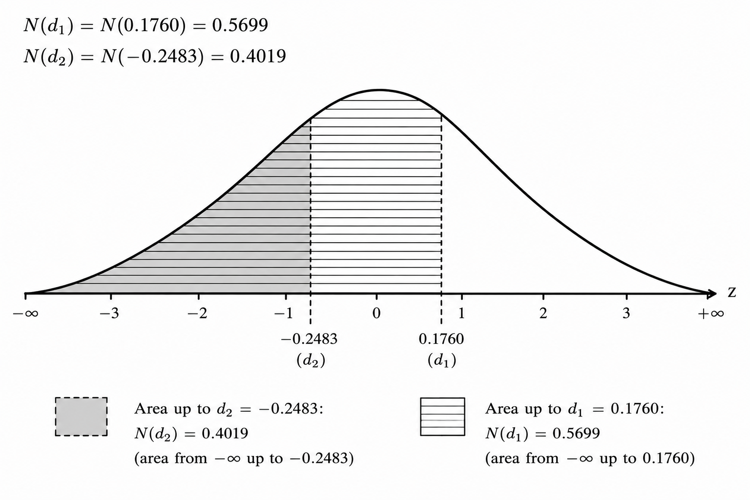
Cumulative Normal Probabilities
Using standard statistical tables or Excel's cumulative standard normal distribution functions (=NORM.S.DIST(Z, TRUE)), we look up our target area values:
-
For the Call Option calculations:
- $N(d_1) = N(0.1760) = \mathbf{0.5699}$
- $N(d_2) = N(-0.2483) = \mathbf{0.4019}$
-
For the Put Option calculations (using symmetry metrics):
- $N(-d_1) = N(-0.1760) = 1 - 0.5699 = \mathbf{0.4301}$
- $N(-d_2) = N(0.2483) = 1 - 0.4019 = \mathbf{0.5981}$
Present Value of the Strike Price
We discount the fixed cash liability ($K$) back to present value terms using continuous compounding friction:
Valuation of the European Call Option ($c$)
Plugging our resolved terms back into the primary call formula:
Valuation of the European Put Option ($p$)
Plugging our complementary terms into the primary put formula:
Market Break-Even Intuition
-
Call Option Breakeven: For an investor purchasing this call option to clear a pure profit at expiration, ignoring the time value of money, the stock price must rise above its strike price by more than the upfront premium paid.
$$\text{Call Breakeven} = K + c = \$110 + \$16.18 = \mathbf{\$126.18}$$The stock must rise from its current price of $\$100$ by a total of **$\$26.18$** to break even. -
Put Option Breakeven: For an investor buying this put option, the asset must drop low enough below the strike to cover the premium expense.
$$\text{Put Breakeven} = K - p = \$110 - \$17.72 = \mathbf{\$92.28}$$The stock must fall from its current price of $\$100$ by a total of **$\$7.72$** to break even.
5.3 Employee Stock Option Valuation
A company has 1,000,000 existing shares outstanding, with the stock currently trading at a market price of $\$100$ per share. The firm surprises the market by announcing that it is considering granting 250,000 new corporate employee stock options. Each option gives the holder the right to buy one share of stock with a strike price of $\$110$ in 2 years ($T = 2.0$).
Using the explicit Black-Scholes-Merton calculations from Example 5.2 , the value of a regular, standard exchange-traded call option on this stock ($c_{\text{regular}}$) is $\mathbf{\$16.18}$. The company pays no dividends, and the market perceives no immediate strategic or operational benefits from this option grant.
- Calculate the fair market value of each individual employee stock option.
- Calculate the total cost of the proposed employee stock option grant to the firm.
- Calculate the immediate post-announcement expected drop in the stock price and the resulting new stock equilibrium price.
From the problem statement, we isolate our core dilution and baseline pricing parameters:
- Number of Existing Shares ($N$): $1,000,000$
- Current Stock Price ($S_0$): $\$100$
- Number of New Contemplated Options ($M$): $250,000$
- Option Strike Price ($K$): $\$110$
- Time to Maturity ($T$): $2.0 \text{ years}$
- Value of a Regular Call Option ($c_{\text{regular}}$): $\$16.18$ (Derived in Section 5.2 at a 4% risk-free rate)
Value of an Individual Employee Stock Option
As derived in the corporate option dilution framework, the value of a single dilutive stock option is equal to a specific structural fraction ($\frac{N}{N + M}$) multiplied by the price of an equivalent, regular exchange-traded call option:
Substituting our parameters into the fraction:
Each individual employee stock option has a fair corporate market value of $\$12.94$.
Total Cost of the Proposed Grant
The total capital cost of this option liability to the firm is the value of each employee option multiplied by the total volume of new contracts granted ($M$):
Stock Price Dilution and New Equilibrium Price
Because the market perceives no immediate operational benefits or salary-saving compensation from this announcement, the aggregate equity value of the firm drops by the exact cost of the issue.
First, we determine the immediate drop or reduction in the stock price:
Alternative Shortcut check using our coefficient formula: $$\frac{M}{N + M} \times c_{\text{regular}} = \frac{250,000}{1,250,000} \times \$16.18 = 0.20 \times \$16.18 = \$3.236$$ The result matches perfectly.
Finally, we subtract this dilution shock from our pre-announcement baseline stock price to find the new market equilibrium:
5.4 Income Statement Impact (During the Vesting Period)
When employee stock options are granted, accounting standards (US GAAP ASC 718 / IFRS 2) require the company to recognize the value of the options as an operating expense. This expense is spread out over the designated vesting period (the time employees must remain with the firm to officially earn the options).
Assuming a 2-year straight-line vesting period, the company must record half of the total liability as an expense each year:
Here is how this entry shifts the primary Income Statement line items:
| Income Statement Line Item | Amount | Notes / Impact |
|---|---|---|
| Revenues | $50,000,000 | |
| Cost of Goods Sold (COGS) | ($30,000,000) | |
| Gross Profit | $20,000,000 | |
| Operating Expenses: | ||
| Salaries and Wages | $5,000,000 | Normal cash compensation |
| Stock-Based Compensation Expense | $1,618,000 | Non-cash operating hit (BSM Engine) |
| Other SG&A | $2,382,000 | |
| Operating Income (EBIT) | $11,000,000 | |
| Net Income | Drops | Reduced by $1,618,000 each year |
Appendix
Numerical Example of Market Efficiency and Dilution
To understand how the market absorbs dilution costs instantly, consider a company possessing the following initial setup:
- Existing Shares ($N$): $100,000$
- Initial Share Price ($S_0$): $\$50$
- Total Equity Value ($N S_0$): $\$5,000,000$
The company surprises the market by announcing that it is granting $100,000$ new stock options ($M = 100,000$) to its employees with a strike price ($K$) of $\$50$.
The Announcement Effect
Suppose the market sees very little structural benefit coming to the shareholders from this option grant (i.e., there are no corresponding salary reductions or measurable increases in managerial motivation). Because this issue represents a net expense, the share price will decline immediately upon the announcement.
If the market prices this future liability and causes the stock price to drop to $\$45$, the dilution cost is absorbed upfront:
- Dilution Cost per Share: $\$50 - $\$45 = \$5$ per share
- Total Cost to Current Shareholders: $100,000 \text{ shares} \times \$5 = \$500,000$
The Fallacy of Second Dilution at Maturity
Now, suppose the company performs well over the next three years, and by the maturity date ($T$), the market share price stands at $\$100$. At this exact point, all $100,000$ employee options are exercised. Because the stock is trading at $\$100$ and the employees pay the strike price of $\$50$, the actual payoff delivered to the employees is $\$50$ per option.
It is highly tempting for students to argue that a second wave of dilution must happen at this moment. The flawed argument usually looks like this:
- Flawed Logic: "We are taking $100,000$ original shares worth $\$100$ each and merging them with $100,000$ new shares for which only $\$50$ was paid. Therefore:
- (a) The post-exercise share price must drop to: $\frac{\$100 + \$50}{2} = \$75$.
- (b) The actual payoff received by the option holder is only: $\$75 - \$50 = \$25$ per option."
Why this Argument is Flawed
This double-counting logic is completely incorrect because an efficient market anticipates the exercise event. The terminal market price of $\$100$ already accounts for the fact that $100,000$ new shares are about to enter the float at $\$50$. If the options had magically been canceled instead of exercised, the stock price would have jumped up even higher.
The true, un-diluted value of the company's underlying assets at maturity is actually $\$150$ per share. The observed market price of $\$100$ is already the clean, diluted equilibrium price. Therefore, the actual payoff from each option exercised remains exactly $\$50$.
This example perfectly illustrates the overarching principle of option pricing: When markets are efficient, the entire impact of dilution from executive stock options or warrants is fully priced into the stock immediately upon their public announcement. It is a capital structure variable that is absorbed upfront, meaning it does not need to be adjusted for or taken into account a second time when calculating the mathematical value of the options.
References
- Hull, J. C. Options, Futures, and Other Derivatives. Pearson. (Explaining standard exchange-traded option valuation algorithms and corporate warrant adjustments).
- Shreve, S. E. Stochastic Calculus for Finance II: Continuous-Time Models. Springer Finance. (Providing the foundational continuous-time martingales and asset drift probability boundaries under the risk-neutral measure).
- Wilmott, P., Howison, S., & Dewynne, J. The Mathematics of Financial Derivatives: A Student Introduction. Cambridge University Press. (Detailing partial differential equation implementations for specialized corporate equity constructs).