Valuation of Stock Option Using Balck-Scholes Model - Part 4

May 19, 2026

4.1 Boundary Conditions and Option Types

We derived the foundational Black–Scholes–Merton differential equation in Section 3.4:

The BSM differential equation has infinite possible mathematical solutions. This means that by itself, the equation does not tell us the price of an option. The specific derivative price obtained when solving the differential equation depends entirely on the boundary conditions that are applied.

These boundary conditions specify the exact value of the derivative contract at the expiration boundaries of possible asset values $S$ and time parameters $t$.

4.1.1 European Call Option Boundary Condition

In the case of a standard European call option, the contract gives the holder the right to buy the asset for strike price $K$ at maturity time $T$. Therefore, the key boundary condition at expiration ($t = T$) is defined by its final payoff function:

4.1.2 European Put Option Boundary Condition

Similarly, a European put option gives the holder the right to sell the underlying stock for the strike price $K$ at maturity time $T$. To price a put contract using the exact same differential equation framework, we simply swap out the call parameters for the put payoff boundary condition at expiration ($t = T$):

By solving the universal BSM partial differential equation subject to these unique terminal boundaries, we can isolate the explicit pricing formulas for both calls and puts.

4.2 Derivation of the BSM Formulas

We can derive the final European call option pricing formula, $c = S_0 N(d_1) - K e^{-rT} N(d_2)$, using a powerful alternative framework: the Risk-Neutral Valuation principle. Instead of solving the partial differential equation via complex calculus transforms, we rely on financial logic: in a risk-neutral world, the expected return on any asset is the risk-free rate $r$.

In a risk-neutral world, the current value of a European call option ($c$) is simply the expected value ($E$) of its terminal payoff, $\max(S_T - K, 0)$, discounted back to the present day at the risk-free interest rate $r$:

To understand the economic logic behind this starting equation, we can break down each individual component:

• $c$: The current, fair market price of the European call option today (at time $t = 0$).
• $\max(S_T - K, 0)$: This is the payoff function of the call option at expiration (time $T$).
  • $S_T$: The random, future stock price at maturity.
  • $K$: The fixed strike price agreed upon in the contract.
  • Note: If the stock price finishes higher than the strike ($S_T > K$), the option is worth the difference ($S_T - K$). If it finishes lower, the option expires worthless ($0$).
• $E[\dots]$: This denotes the mathematical expectation (the average expected outcome) calculated under a risk-neutral probability distribution.
• $e^{-rT}$: The continuous discount factor. It scales the future cash value back to present-day dollars using the annualized risk-free interest rate ($r$) over the time horizon ($T$).

Because this expected payoff only generates a positive value when the terminal stock price finishes above the strike price ($S_T > K$), we can represent this expectation as a continuous integral using the probability density function $f(S_T)$ from $K$ to $\infty$:

To evaluate this systematically, we split the expression into two separate functional component integrals:

Deriving Term 2 (The Probability of Exercise, $N(d_2)$)

Let's solve Term 2 first, as its probability translation is highly intuitive. The integral component $\int_{K}^{\infty} f(S_T) dS_T$ represents the literal probability that the option finishes in-the-money and will be exercised, written as $P(S_T > K)$.

Because a stock price ($S$) cannot fall below zero, the Black–Scholes–Merton model assumes that the natural logarithm of the stock price ($\ln S$) follows a normal distribution. In a risk-neutral world, the log terminal stock price at maturity has the following parameters:

• Mean ($\mu$): $\ln S_0 + \left(r - \frac{\sigma^2}{2}\right)T$
• Standard Deviation: $\sigma\sqrt{T}$

Recall from standard statistics that the universal formula used to standardize a normal random variable $X$ into a Z-score is:

We begin by defining our target probability boundary condition:

Our core goal is to find the probability that the terminal stock price ($S_T$) ends up higher than the strike price ($K$). Because taking the natural logarithm ($\ln$) on both sides of an inequality preserves its direction, we apply it to map our absolute asset prices into log-space variables.

This is the central step of the derivation. To convert our log-space variables into standard units, we subtract the risk-neutral mean from both sides, and then divide both sides by the standard deviation:

Now that the left-hand side of our inequality has been simplified to the standard normal variable $Z$, we focus on simplifying the numerator on the right-hand side. Let's isolate the numerator terms:

Distributing the negative sign across the brackets yields:

Using the fundamental logarithmic subtraction property ($\ln A - \ln B = \ln(A/B)$), we can combine the initial log terms:

Placing this simplified numerator back over our standard deviation denominator ($\sigma\sqrt{T}$) brings us directly to the next line of the textbook proof structure:

Currently, our probability equation calculates an upper-bound tail area:

However, the final Black–Scholes–Merton formula relies on standard cumulative probability notation, $N(d)$, which by definition measures a left-tailed cumulative baseline ($P(Z < d)$).

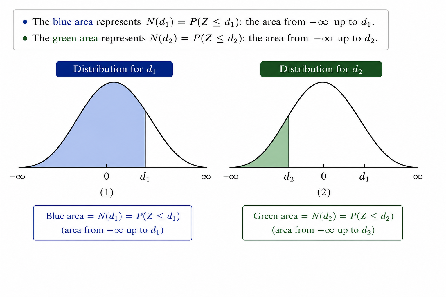
Because a standard normal bell curve is perfectly symmetric around a mean of zero, the probability of being greater than a specific negative threshold is identical to the probability of being less than that same threshold flipped to a positive sign. Mathematically, this identity states that $P(Z > -d_2) = P(Z < d_2) = N(d_2)$.

To apply this symmetry mapping, we multiply the entire right-hand side fraction by $-1$ and flip the inequality sign:

• Multiplying $\ln(K/S_0)$ by $-1$ yields $-\ln(K/S_0)$, which flips into $\ln(S_0/K)$.
• Multiplying $-\left(r - \frac{\sigma^2}{2}\right)T$ by $-1$ flips the sign into $+\left(r - \frac{\sigma^2}{2}\right)T$.

This sign inversion isolates our explicit target parameter $d_2$:

As a result, this entire conditional probability expression cleans up directly into our final notation:

Therefore, Term 2 of our option pricing equation resolves to the present value of the expected cash payment at strike price $K$:

Deriving Term 1 (The Expected Asset Value Received, $S_0 N(d_1)$)

Term 1 serves as the mathematical foundation for evaluating the present value of the expected stock shares received upon exercise ($e^{-rT} E[S_T \text{ given } S_T > K]$).

To understand how this complex, continuous integral simplifies into the elegant expression $S_0 N(d_1)$, we apply statistical variable substitution alongside algebraic completion of the square.

We begin with the raw operational definition of Term 1:

• $e^{-rT}$: The continuous temporal discount factor that scales future cash-equivalent terminal values back to present-day value.
• $\int_{K}^{\infty}$: The operational boundaries of integration. Because a call option is only exercised if the terminal stock price exceeds the strike price ($S_T > K$), we evaluate our density domain from the baseline $K$ to $\infty$.
• $S_T$: The absolute price of the underlying stock at maturity time $T$.
• $f(S_T)$: The lognormal probability density function (PDF) tracking the random distribution path of the terminal stock price.

Logarithmic Variable Substitution ($x = \ln S_T$)

To make this expression workable, we map our absolute stock variables into standard log-space by defining $x = \ln S_T$:

• This definition implies that $S_T = e^x$.
• Differentiating both sides yields $\frac{1}{S_T} dS_T = dx$, which means $dS_T = S_T \, dx = e^x \, dx$.
• The lower integration boundary shifts from $K$ into $\ln K$.

Substituting these properties back into our core integral removes the raw asset variables. For algebraic simplicity throughout the next two steps, let's define our risk-neutral log mean parameter as $m = \ln S_0 + \left(r - \frac{\sigma^2}{2}\right)T$ and the absolute log standard deviation parameter as $v = \sigma\sqrt{T}$:

Combining the Exponential Terms

Inside our integration window, we have two distinct exponential functions multiplied together: $e^x$ and $\exp\left(-\frac{(x-m)^2}{2v^2}\right)$. Using standard laws of exponents ($e^A \cdot e^B = e^{A+B}$), we combine their powers:

We isolate our variable $x$ by completing the square inside the numerator:

We place this restructured exponent back inside our integration window. Because the constant addition term $\exp\left(m + \frac{v^2}{2}\right)$ does not contain our tracking variable $x$, we factor it completely outside of the integral:

Let's analyze the external exponential multipliers sitting outside our integral window:

Now, let's substitute our original definitions for the mean ($m$) and variance ($v^2$) directly back into this exponent:

Notice that a flawless algebraic cancellation occurs: $-rT$ and $+rT$ neutralize each other completely, while $-\frac{\sigma^2 T}{2}$ and $+\frac{\sigma^2 T}{2}$ destroy each other as well. This leaves us with:

Remarkably, all of the complex volatility drag components and temporal discounting factors outside the integral collapse down to the current spot price of our stock, $S_0$!

Next, we isolate and resolve our remaining integral equation:

This is the probability density function of a normal distribution possessing a modified mean of $(m + v^2)$ and a standard deviation of $v$. To calculate the area from $\ln K$ to $\infty$, we transform this variable into a standard normal Z-score ($Z \sim \phi(0, 1)$):

To locate our new lower boundary in standard normal space, we substitute our log-strike baseline $\ln K$ into our tracking variable $x$:

Plugging our explicit baseline parameters ($m$ and $v^2$) back into this expression yields:

This restates our integration problem as finding the upper-tail normal area where $P(Z > -d_1)$. Applying our standard normal distribution curve symmetry identity, the area to the right of a negative threshold matches the cumulative area to the left of its positive counterpart:

Now, we recombine our external spot asset coefficient from Step 4 with our normalized integration term from Step 5:

This completes the derivation for the first half of the Black–Scholes–Merton model. It provides the mathematical proof that the present value of the expected stock asset units received upon exercise simplifies cleanly to the current spot stock price scaled by the metric $N(d_1)$.

Now that both components of our original expectation integral have been fully solved, we can substitute them back into our primary pricing framework.

From equation (4.5), we recall our split integral structure:

Plugging in our finalized expressions—$\text{Term 1} = S_0 N(d_1)$ from Step 3 and $\text{Term 2} = K e^{-rT} N(d_2)$ from Step 2—yields the definitive Black–Scholes–Merton Pricing Formula for a European Call Option:

Where the explicit internal boundary variables are systematically defined as: